
Les meilleurs indicateurs précoces de défaillance ne sont souvent mesurés directement par aucun instrument : ils se calculent à partir de valeurs dont le banc dispose déjà. Une mesure dérivée est l'une de ces valeurs calculées, enregistrée comme une mesure normale, avec son propre nom, son unité et ses limites.
Une fois enregistrée, une mesure dérivée se comporte comme n'importe quelle autre : elle apparaît dans le contrôle des mesures, obtient une carte de contrôle et un Cpk, peut porter des validateurs, s'exporte en CSV et participe aux alertes de dérive. Une valeur qui n'existe que dans une formule de tableur ne fait rien de tout cela.
Prérequis
- Une procédure de test qui enregistre au moins deux mesures liées dans une même phase
Étape 1 : calculer la valeur dans la phase
Dérivez la valeur là où les mesures brutes sont prises, et enregistrez-la dans la même phase :
drops = {}for contact in ["A1", "A2", "A3"]: mv = dmm.measure_dc_millivolts(contact) drops[contact] = mvmeasurements.contact_drop_a1 = drops["A1"]measurements.contact_drop_a2 = drops["A2"]measurements.contact_drop_a3 = drops["A3"]# Dérivée : déséquilibre entre les pôles, un meilleur indicateur# précoce que n'importe quel pôle face à sa propre limite.measurements.contact_drop_spread = round(max(drops.values()) - min(drops.values()), 2)Étape 2 : lui donner une limite
Une mesure dérivée prend toute sa valeur quand elle porte son propre validateur. Dans l'exemple, chaque pôle a une limite de 100 mV, et l'écart reçoit une limite de 40 mV. Une unité peut respecter les trois limites de pôle et échouer malgré tout sur l'écart, ce qui est exactement la classe de défaut que les limites individuelles ne peuvent pas voir.
Fixez la limite à partir des données de la flotte, pas de l'intuition : enregistrez d'abord la mesure sans validateur, observez la distribution saine dans le contrôle des mesures, et placez la limite en dehors de celle-ci.
Étape 3 : choisir des dérivations qui révèlent des modes de défaillance
Schémas utiles :
| Dérivation | Calcul | Ce qu'elle révèle |
|---|---|---|
| Écart | max - min entre canaux | Un canal qui se dégrade parmi des canaux nominalement identiques |
| Marge | limite - valeur mesurée | L'érosion de la réserve avant qu'une limite ne soit franchie |
| Rapport | valeur A / valeur B | Des décalages qui affectent les deux valeurs mais changent leur relation |
| Écart à la référence | valeur - valeur de l'échantillon de référence | Dérive du montage ou de l'instrument |
| Symétrie | gauche - droite, ou phase à phase | Asymétrie mécanique ou de bobinage |
Étape 4 : analyser au niveau de la flotte
Ouvrez le contrôle des mesures et sélectionnez la mesure dérivée sur tout l'historique. Une flotte saine forme une seule population ; un mode de défaut en fait apparaître une seconde :
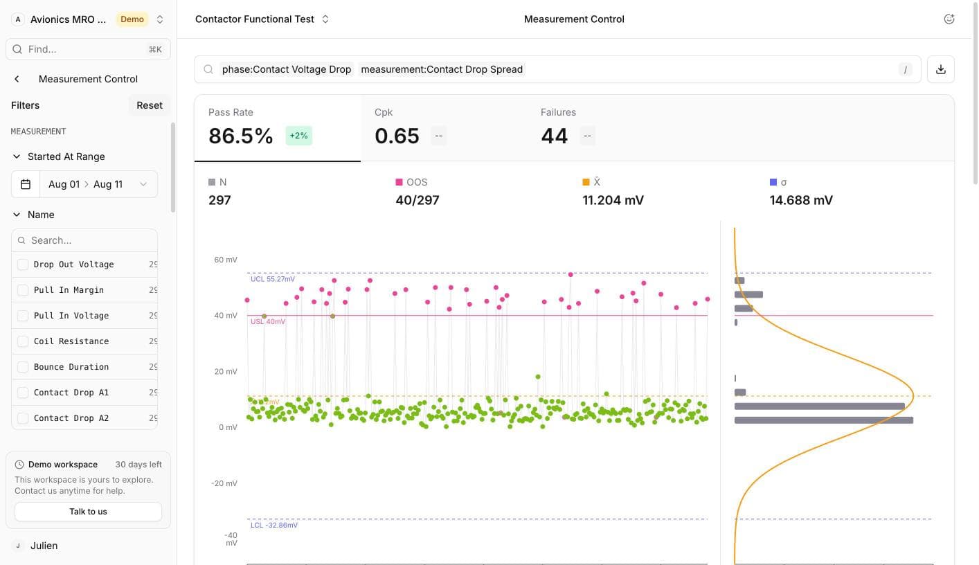
À partir de là, les outils habituels s'appliquent : carte de contrôle, histogramme, Cpk, filtrage par numéro de série et export CSV pour tout ce que vous souhaitez approfondir.