
A latent defect is a unit that passes every individual limit on the bench but fails in service. This guide shows how one derived measurement plus a fleet-level control chart makes that population visible, using a simulated avionics contactor fleet as the worked example.
The pattern matters most in maintenance and repair environments: high mix, low volume, complex degradation. A per-unit OK/NG verdict answers "can this unit ship today", but it says nothing about which passing units are quietly degrading. That signal only exists at fleet level.
Prerequisites
- A test procedure uploading runs to TofuPilot
- A measurement that captures the defect signature (see Step 1)
- Two or more shop visits per unit, so per-serial trends exist
Step 1: Record a signature measurement
Individual limits are set per measurement, so a defect that shifts the relationship between measurements stays invisible to them. Record that relationship as its own measurement.
In the contactor example, each pole's voltage drop has a 100 mV limit. A latent coil defect raises one pole about 45 mV above the others while all three stay under 100 mV. The imbalance between poles is the signature:
# Imbalance between poles is a better early indicator than any single pole.spread = round(max(drops.values()) - min(drops.values()), 2)measurements.contact_drop_spread = spreadGive the derived measurement its own limit (40 mV here). One line in the bench script, and every past and future run carries the signature.
Step 2: Read the fleet distribution
Open measurement control, select the derived measurement over the full history, no other filters.
A healthy fleet produces one population. A fleet with a latent defect mode produces two. In the contactor fleet (150 units, 24 months, 297 measurements), the histogram is bimodal: the healthy body sits near 11 mV, and a second population sits at 42-55 mV, above the 40 mV limit. Cpk on the same view (0.65 here) quantifies what the histogram shows.
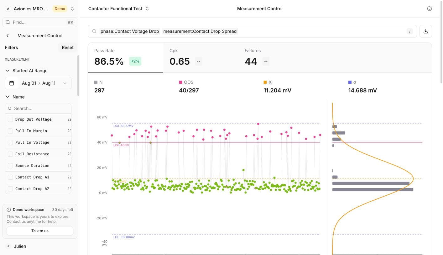
No hypothesis was needed: selecting the measurement is the entire analysis. This is the practical difference from spreadsheet work, where each candidate relationship must be extracted, pivoted, and plotted one at a time.
Step 3: Separate latent from overt units
Filter the measurement outcome to FAIL and compare with the per-pole measurements:
| Population | Definition | Contactor fleet |
|---|---|---|
| Overt | At least one individual limit failing | 14 units |
| Latent | Every individual limit passing, signature over limit | 9 units |
The 9 latent units are the ones a per-pole bench ships. They are also the future no-fault-found cases: removed on a squawk, tested OK on every individual limit, returned to stock.
Step 4: Scope one serial and read the trend
Filter to a single serial with the serial number filter and select the drifting measurement.
On the example unit, pole A2 climbs linearly from 92.5 mV to 104.6 mV across six shop visits as operating hours accumulate, crossing its 100 mV limit between visits four and five. The spread measurement had been over its limit since the first visit, 19 months earlier.
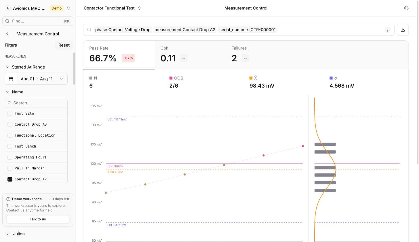
On paper this unit is an intermittent repeat visitor. On the chart it is monotonic degradation with a predictable crossing date, which changes the maintenance decision from "test again and return to stock" to "replace the coil now".
Step 5: Watch for it automatically
Two alert types cover this pattern without manual review:
- A retest threshold alert fires when a unit accumulates repeated tests on the same procedure, which is how no-fault-found loops look in the data.
- A measurement drift alert grades each measurement against its own baseline and fires when the series genuinely moves, catching the per-serial climb of Step 4 as it happens.