
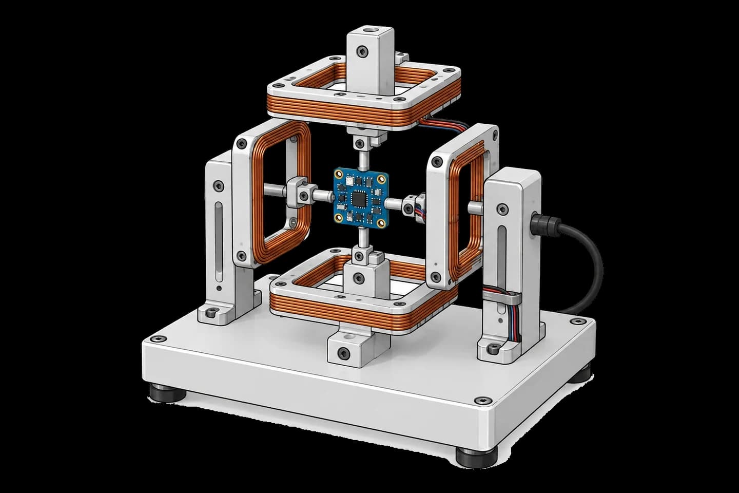
Get the complete source, dependencies and setup instructions from the template repository.
Open the source on GitHubIntroduction
Magnetometer Overview
Magnetometers measure the direction and strength of magnetic fields, and on a drone they provide the absolute heading reference that GPS and IMU fusion cannot give alone. Without a magnetometer, an autopilot can hold attitude but cannot tell north from south once the drone is stationary or moving slowly. Every consumer and industrial multirotor running PX4, ArduPilot, or Betaflight relies on a triaxial magnetometer to anchor yaw and enable features like Return-to-Home, waypoint navigation, and heading hold.
Modern drone magnetometers are MEMS or AMR (Anisotropic Magneto-Resistive) chips that resolve the Earth's magnetic field, which ranges from about 25 µT near the equator to 65 µT near the poles. Typical parts used in production include the QMC5883L (16-bit ADC, 2 mGauss field resolution), the IST8310 (14-bit, up to 200 Hz, 166 Hz in its low-noise 16x-averaging mode), and the MMC5983MA (18-bit, 0.4 mGauss RMS noise, built-in degaussing). Each has different noise floors and bias-drift characteristics, which matters when defining production limits.
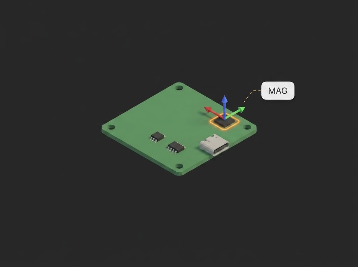
The magnetometer package and its sensor axes on the flight-controller board.
The challenge is that the magnetometer never sees a clean Earth field. The drone itself carries ferromagnetic materials (screws, ESC traces, motor magnets) and current-carrying conductors (battery leads, motor phases) that distort the field at the sensor location. Two distinct error sources result, and both must be characterized per-unit at the end of the production line.
Calibration Purpose
The goal of hard/soft iron calibration is to map the distorted ellipsoidal locus of magnetometer readings back to a clean sphere centered at the origin. When the drone is rotated through all orientations in a uniform magnetic field, raw readings should trace a perfect sphere of radius equal to the local field magnitude. In practice they trace an off-center, rotated ellipsoid because of two effects:
- Hard iron distortion: additive bias from permanently magnetized materials on the airframe (motor magnets, magnetized screws). Shifts the sphere center away from the origin without changing its shape.
- Soft iron distortion: multiplicative scale and skew from ferromagnetic materials (steel mounts, battery casing) that reshape the ambient field. Stretches the sphere into an ellipsoid.
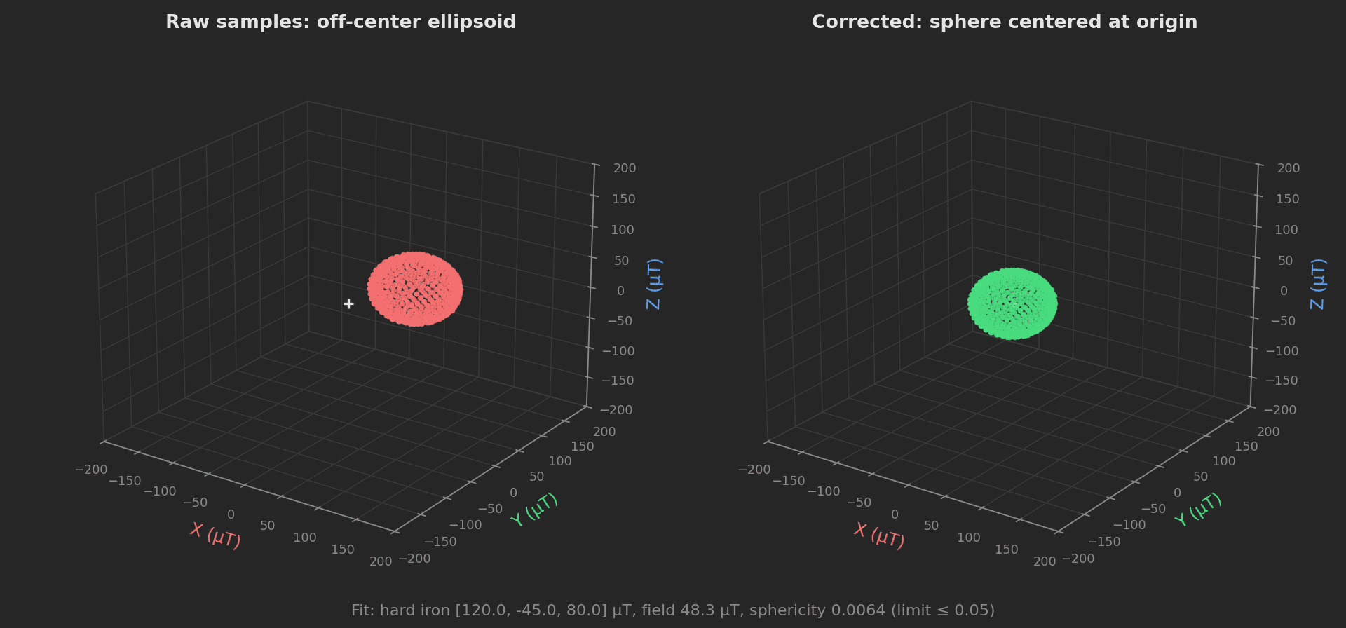
Raw samples from the mock DUT and the same samples after applying the fitted hard and soft iron correction.
The calibration produces two artifacts per drone: a 3-element offset vector (hard iron) and a 3x3 transformation matrix (soft iron). At runtime, every raw reading m_raw is corrected as m_cal = SoftIron · (m_raw - HardIron) before being passed to the attitude estimator. These parameters are unique to each airframe and must be written to non-volatile storage on the flight controller (in PX4 this means the CAL_MAG0_* parameters written to /fs/mtd_caldata during factory calibration).
Per-unit factory calibration addresses a leading source of consumer drone field returns: erratic compass behavior leading to fly-aways, toilet-bowling, and failed Return-to-Home. The procedure adds 60-90 seconds to end-of-line testing.
This template also serves as a working tour of several TofuPilot Framework capabilities: live operator UI updates during acquisition, automatic phase retry when coverage is insufficient, a JSON measurement holding the calibration coefficients, numeric-array aggregations, an interactive residual chart, and a raw-data attachment.
Equipment & Setup
To implement hard/soft iron calibration for a drone magnetometer on a production line, the following equipment is required:
- A magnetically clean test cell: area free of moving ferromagnetic objects within 1 m of the DUT, with stable ambient field (or active cancellation if the building has structural steel).
- A controlled rotation mechanism: either a 3-axis motorized gimbal, a turntable with operator-guided tilt, or a calibrated handheld procedure with a visual coverage UI.
- A reference magnetometer for ambient field verification, typically a high-stability fluxgate.
- The Device Under Test (DUT) equipped with the magnetometer to be calibrated, mounted in the same orientation as in the final airframe.
- Firmware with a triggerable raw-mag streaming mode (no on-chip filtering, no fusion corrections applied).
- A TofuPilot Framework procedure to acquire samples, fit the ellipsoid, validate the result, and write parameters back to the DUT.
- The TofuPilot Dashboard to store calibration parameters for traceability, monitor 3σ drift across the production batch, and trace each unit by serial.
Hardware Components
Helmholtz Coil (Optional, Deterministic Setup)
For high-volume or high-accuracy production, a 3-axis Helmholtz coil generates a known, uniform magnetic field around the DUT and removes dependency on ambient conditions. The Bartington HC2 (1 m nominal coil diameter, field homogeneous to better than 0.1% over a 13.6 cm cube at the center) fits drone-sized boards comfortably, paired with a Mag-03 fluxgate reference to verify field stability. The Helmholtz approach allows the DUT to remain stationary while the field is rotated electronically through known vectors, making the procedure deterministic and fully scriptable.
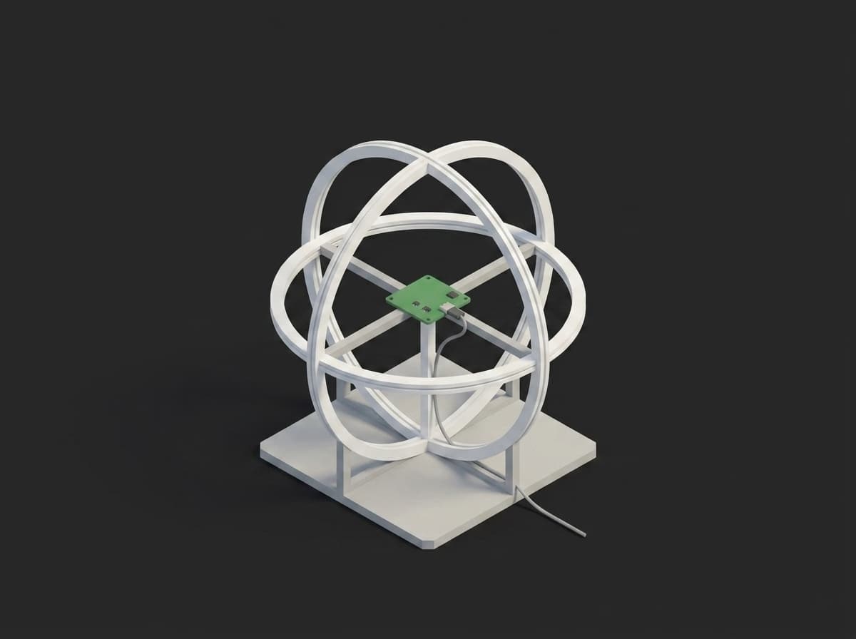
Three-axis Helmholtz coil with the PCBA at the homogeneous center.
Note that Helmholtz coil systems need roughly 30 minutes of warm-up, and the field at the DUT location must be verified with the reference magnetometer before each shift. For most consumer drone lines, the simpler Earth-field method below is sufficient.
Earth-Field Rotation Jig (Default Setup)
Most production lines calibrate against the local Earth magnetic field, which is stable to a fraction of a percent on magnetically quiet days at a fixed location. The DUT is mounted on a non-magnetic (aluminum or 3D-printed) jig and either rotated by an operator following a UI prompt, or by a 3-axis motorized stage that runs a fixed coverage pattern.
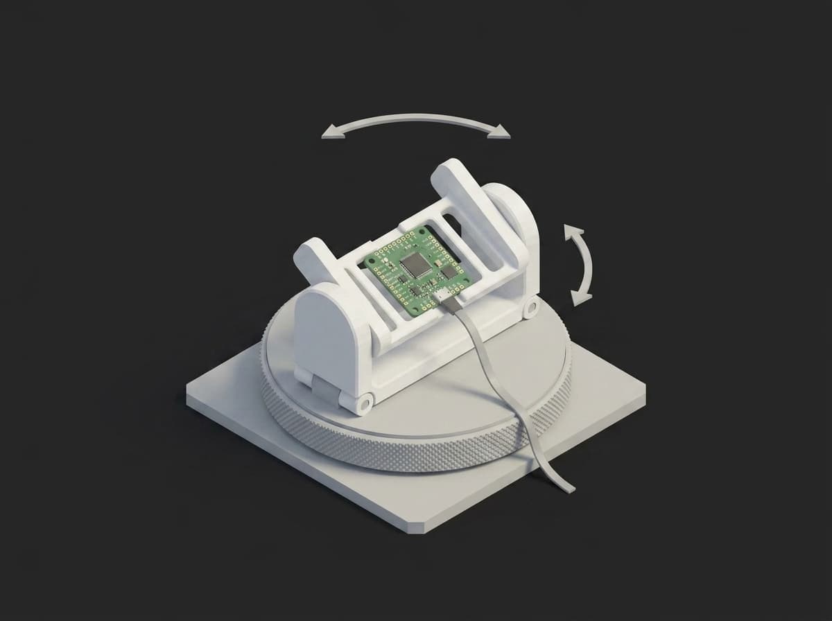
Two-axis 3D-printed cradle on a turntable: tilt plus rotation covers the sphere.
The jig must be mounted away from the test bench's steel frame (typical 30 cm clearance), and operators must be instructed not to wear steel-toed boots or magnetic badge clips near the test cell.
Reference Magnetometer
A Bartington Mag-03 triaxial fluxgate (±70 µT lowest range, noise floor under 10 pT/√Hz at 1 Hz) is the production standard for verifying the local field magnitude before each batch. The reference reading establishes the target sphere radius for ellipsoid fitting: if the corrected drone readings don't sit on a sphere of this radius, calibration has failed regardless of fit residual.
Custom Firmware
The DUT firmware must expose a raw streaming mode that bypasses any on-chip averaging, soft-iron correction, or fusion filtering. During calibration the procedure logs:
- Timestamp (ms precision)
- Raw magnetometer X/Y/Z in µT (or ADC counts with known LSB scale)
- Temperature (used to flag thermal drift during calibration, and to disqualify samples taken during warm-up)
- Orientation hint (quaternion from the IMU's gyro+accel fusion), used by the UI to track coverage
Sample rate should be 50-100 Hz; the algorithm needs a few hundred well-distributed samples, which takes 30-60 seconds at human rotation speed. PX4's onboard calibration procedure (operator-rotated, all-orientation coverage) is a good reference baseline.
Test Procedure
Overview
The procedure runs two phases:
- Acquire Samples: pull raw samples from the DUT while the operator rotates it, show live coverage feedback, and retry the acquisition if orientation coverage is insufficient.
- Fit Calibration: fit the ellipsoid, validate offsets and residuals, attach the raw data, and save the calibration to the DUT.
Why TofuPilot Framework?
TofuPilot Framework is a YAML + Python test framework built for hardware manufacturing. Instead of writing all your test logic, measurements, and limits inside Python code, you describe what the test does in a procedure.yaml file, and how in small Python phase files. The framework handles:
- Automatic Python environment management (via
uv) - Operator UI (no frontend code needed)
- Measurement validation and live charts
- Process isolation between phases and equipment plugs
Project Structure
You can find the full source on GitHub. Run it locally with tofupilot run .; the mock plug synthesizes samples so no hardware is needed.
The Procedure File
procedure.yaml declares the procedure identity, the unit (auto-identified from defaults, so the run starts without operator input), and the mock DUT plug. The Dashboard ID for automatic upload lives in this same file once the procedure is linked:
name: Magnetometer Hard/Soft Iron Calibrationversion: 0.1.0description: Acquires magnetometer samples across all orientations, fits an ellipsoid to estimate hard and soft iron distortion, validates residuals, and saves the calibration.unit: auto_identify: true serial_number: default_value: "SN00001" part_number: default_value: "FC-MAG-01"plugs: - name: Mock DUT description: Simulated flight controller streaming raw magnetometer samples. python: plugs.mock_dut:MockDut key: dutAcquisition with Live UI and Retry
The acquisition phase declares two display components and a retry policy. While Python runs, it pushes coverage updates straight to the operator screen by assigning to ui.<key>. If coverage lands below the target, the phase calls phase.retry() and the framework re-runs it, up to the declared limit, with each attempt recorded on the dashboard:
procedure.yaml25 lines
main: - name: Acquire Samples key: acquire_samples python: phases.acquire_samples retry: limit: 3 delay: 1s ui: components: - key: rotation_progress type: progress label: "Rotation Coverage" default_value: 0 - key: status type: text label: "Status" default_value: "Waiting for samples..." measurements: - name: Coverage key: coverage_pct unit: "%" description: Fraction of orientation bins hit during the tumble. validators: - operator: ">=" expected_value: 80phases/acquire_samples.py31 lines
from utils.coverage import compute_coverageSAMPLE_COUNT = 600COVERAGE_TARGET = 80.0def acquire_samples(dut, measurements, ui, phase, log): """Pull raw samples from the DUT and check orientation coverage. Display components update live while the acquisition runs. If the operator missed too many orientations, the phase asks for another tumble and retries. """ ui.status = "Acquiring samples, rotate the drone through all orientations..." ui.rotation_progress = 10 samples = dut.acquire_samples(SAMPLE_COUNT) log.info(f"Acquired {len(samples)} samples") ui.rotation_progress = 60 coverage = compute_coverage(samples) measurements.coverage_pct = coverage ui.rotation_progress = int(coverage) if coverage < COVERAGE_TARGET: ui.status = f"Coverage {coverage:.0f}% is below {COVERAGE_TARGET:.0f}%, rotate around more axes" log.warning(f"Insufficient coverage ({coverage:.1f}%), retrying acquisition") phase.retry() ui.status = f"Coverage {coverage:.0f}%, acquisition complete" log.info(f"Coverage {coverage:.1f}%")The mock DUT simulates the classic operator mistake on the first attempt (rotation around a single axis) so the retry path actually executes: attempt 1 measures ~23% coverage and retries, attempt 2 tumbles the full sphere and passes at 100%.
Coverage Validation
Ellipsoid fitting requires samples distributed across all orientations. A common production failure is operators rotating only around two axes, leaving a coverage gap that produces a degenerate fit. We bin the sample directions against a Fibonacci sphere grid and require at least 80% of bins hit before proceeding:
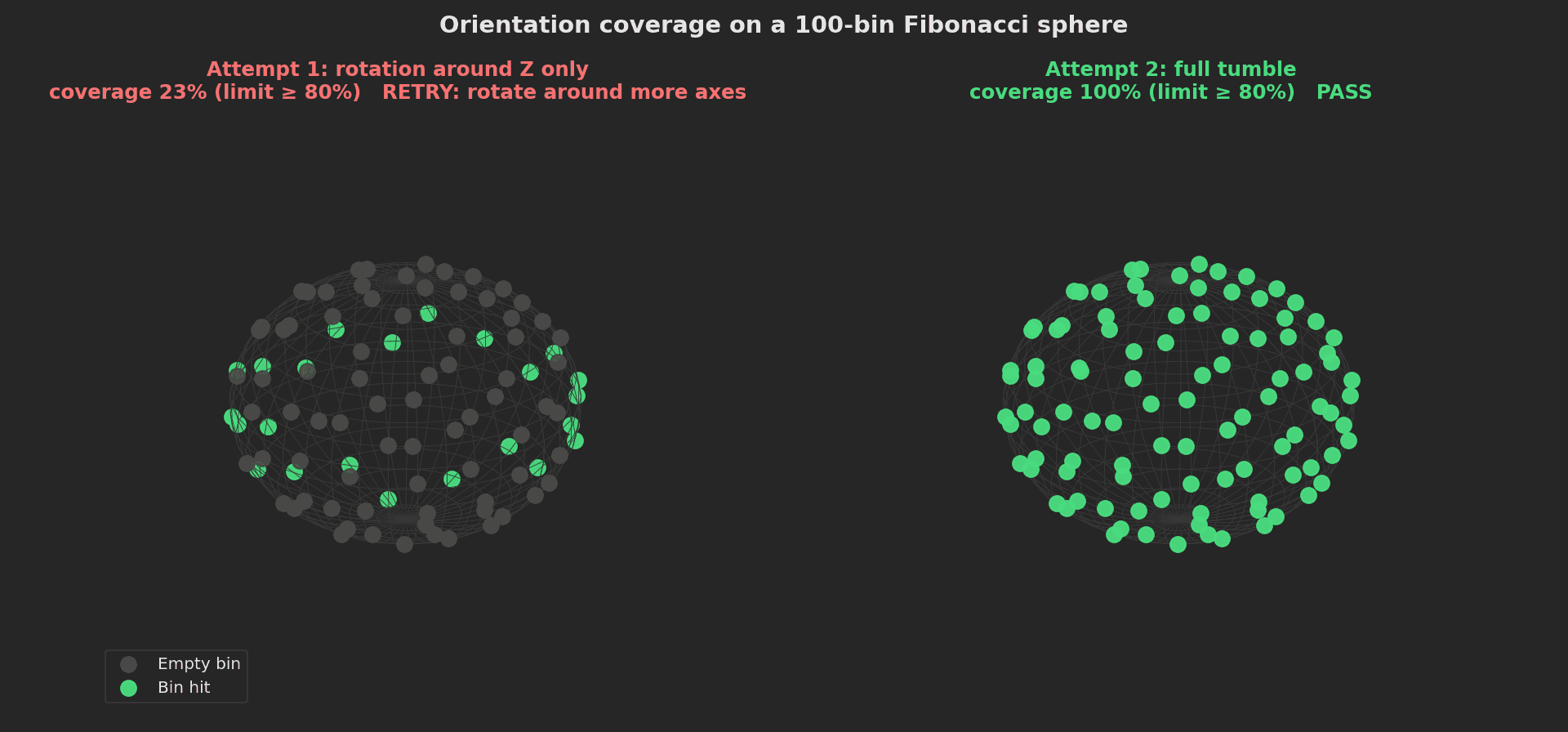
Coverage bins hit by the mock's two attempts, on the same 100-bin grid the phase uses.
utils/coverage.py24 lines
import numpy as npdef compute_coverage(samples, bins=100): """Fraction of orientation bins hit by the sample set, in percent. Bins are directions on a Fibonacci sphere; each sample counts toward its nearest bin. Rotating around a single axis leaves most bins empty, which is the classic operator mistake this check catches. """ samples = np.asarray(samples, dtype=float) centered = samples - samples.mean(axis=0) norms = np.linalg.norm(centered, axis=1) directions = centered[norms > 1e-9] / norms[norms > 1e-9, None] i = np.arange(bins) phi = np.arccos(1.0 - 2.0 * (i + 0.5) / bins) theta = np.pi * (1.0 + 5.0**0.5) * i grid = np.column_stack( [np.sin(phi) * np.cos(theta), np.sin(phi) * np.sin(theta), np.cos(phi)] ) nearest = np.argmax(directions @ grid.T, axis=1) return 100.0 * len(np.unique(nearest)) / binsEllipsoid Fitting
The core algorithm fits a general quadric to the raw 3D points:
a·x² + b·y² + c·z² + 2f·yz + 2g·xz + 2h·xy + 2p·x + 2q·y + 2r·z = 1
This is solved via least-squares decomposition of the 9-parameter system (Renaudin et al., 2010 is the canonical reference). The resulting quadric is decomposed via eigenvalue analysis into the hard iron offset (ellipsoid center) and the soft iron matrix that maps the ellipsoid back onto a sphere:
utils/fit_ellipsoid.py44 lines
import numpy as npdef fit_ellipsoid(samples): """Least-squares quadric fit of magnetometer samples. Fits a*x^2 + b*y^2 + c*z^2 + 2f*yz + 2g*xz + 2h*xy + 2p*x + 2q*y + 2r*z = 1, then decomposes the quadric into a hard iron offset (ellipsoid center) and a soft iron correction matrix that maps the ellipsoid back onto a sphere. Returns (offset, soft_iron, field_strength) where corrected = soft_iron @ (raw - offset) lies on a sphere of radius field_strength. """ s = np.asarray(samples, dtype=float) x, y, z = s[:, 0], s[:, 1], s[:, 2] design = np.column_stack( [x * x, y * y, z * z, 2 * y * z, 2 * x * z, 2 * x * y, 2 * x, 2 * y, 2 * z] ) coeffs, *_ = np.linalg.lstsq(design, np.ones_like(x), rcond=None) a, b, c, f, g, h, p, q, r = coeffs quadric = np.array([[a, h, g], [h, b, f], [g, f, c]]) linear = np.array([p, q, r]) offset = -np.linalg.solve(quadric, linear) # Radius^2 of the centered quadric: x^T Q x = 1 + offset^T Q offset k = 1.0 + offset @ quadric @ offset evals, evecs = np.linalg.eigh(quadric / k) radii = 1.0 / np.sqrt(evals) field_strength = float(np.prod(radii) ** (1.0 / 3.0)) # Map the ellipsoid onto a sphere of radius field_strength. whitening = evecs @ np.diag(np.sqrt(evals)) @ evecs.T soft_iron = field_strength * whitening return offset, soft_iron, field_strengthdef apply_calibration(samples, offset, soft_iron): s = np.asarray(samples, dtype=float) return (s - offset) @ np.asarray(soft_iron).TRunning against the mock data (true offset [120, -45, 80] µT, 48 µT field, 0.3 µT noise), the fit recovers [120.0, -45.0, 80.0] µT and a field strength of 48.3 µT.
Calibration Phase
The second phase fits the ellipsoid, records every artifact, and saves the result. The framework injects dut, measurements, attach, and log by matching parameter names. The full coefficient set is stored as a JSON measurement, the corrected magnitudes as a numeric array with aggregations, the residuals as an interactive multi-dimensional chart, and the raw samples as a CSV attachment via attach.data():
phases/fit_calibration.py61 lines
import ioimport numpy as npfrom utils.fit_ellipsoid import apply_calibration, fit_ellipsoiddef fit_calibration(dut, measurements, attach, log): """Fit the ellipsoid, validate residuals, and save the calibration.""" samples = np.asarray(dut.get_last_samples()) offset, soft_iron, field = fit_ellipsoid(samples) log.info( f"Hard iron offset: [{offset[0]:.1f}, {offset[1]:.1f}, {offset[2]:.1f}] µT, " f"field {field:.1f} µT" ) measurements.offset_x = float(offset[0]) measurements.offset_y = float(offset[1]) measurements.offset_z = float(offset[2]) # JSON measurement: the exact coefficients written to the DUT. measurements.calibration_coefficients = { "hard_iron_ut": [round(float(v), 3) for v in offset], "soft_iron": [[round(float(v), 5) for v in row] for row in soft_iron], "field_strength_ut": round(field, 3), } corrected = apply_calibration(samples, offset, soft_iron) magnitudes = np.linalg.norm(corrected, axis=1) measurements.sphericity_ratio = float(magnitudes.std() / magnitudes.mean()) # Numeric array with aggregations validated by the framework. measurements.field_magnitude = magnitudes.tolist() measurements.field_magnitude.aggregations.mean = float(magnitudes.mean()) measurements.field_magnitude.aggregations.std = float(magnitudes.std()) # Multi-dimensional chart: residual per sample, rendered interactively. residuals = magnitudes - field chart = measurements.residual_chart chart.x_axis = list(range(len(residuals))) chart.y_axis.residual = residuals.tolist() aggs = chart.y_axis.residual.aggregations aggs.mean = float(residuals.mean()) aggs.std = float(residuals.std()) aggs.p2p = float(np.ptp(residuals)) # Attach the raw samples for offline analysis. buffer = io.StringIO() buffer.write("mag_x_ut,mag_y_ut,mag_z_ut") for row in samples: buffer.write(f"{row[0]:.3f},{row[1]:.3f},{row[2]:.3f}") attach.data(buffer.getvalue().encode(), "raw_samples.csv") dut.save_calibration( [float(v) for v in offset], [[float(v) for v in row] for row in soft_iron] ) log.info("Calibration saved to DUT")Parameter Validation
Per-axis bounds derived from the magnetometer datasheet are declared as validators in procedure.yaml, then refined via TofuPilot 3σ analytics over the first batch:
- Hard iron offset per axis: typically within ±300 µT. A value above this suggests a magnetized screw or rework defect.
- Sphericity ratio (std of corrected magnitudes over their mean): a perfect calibration gives < 0.02; production limit 0.05.
- Residual chart aggregations: mean near zero, std and peak-to-peak bounded.
The YAML below shows the X-axis offset; offset_y and offset_z are declared identically:
procedure.yaml58 lines
measurements: - name: Hard Iron Offset X key: offset_x unit: µT validators: - operator: ">=" expected_value: -300 - operator: "<=" expected_value: 300 - name: Sphericity Ratio key: sphericity_ratio description: Std of corrected magnitudes divided by their mean. validators: - operator: "<=" expected_value: 0.05 - name: Calibration Coefficients key: calibration_coefficients description: Hard iron offset vector and soft iron matrix written to the DUT. - name: Corrected Field Magnitude key: field_magnitude unit: µT aggregations: - type: mean unit: µT validators: - operator: ">=" expected_value: 20 - operator: "<=" expected_value: 70 - type: std unit: µT validators: - operator: "<=" expected_value: 1.0 - name: Residual Chart key: residual_chart title: Corrected Magnitude Residual x_axis: legend: Sample y_axis: - legend: Residual key: residual unit: µT aggregations: - type: mean validators: - operator: ">=" expected_value: -0.5 - operator: "<=" expected_value: 0.5 - type: std validators: - operator: "<=" expected_value: 1.0 - type: p2p validators: - operator: "<=" expected_value: 6.0The interactive residual chart replaces the static PNG plot you would otherwise attach manually:
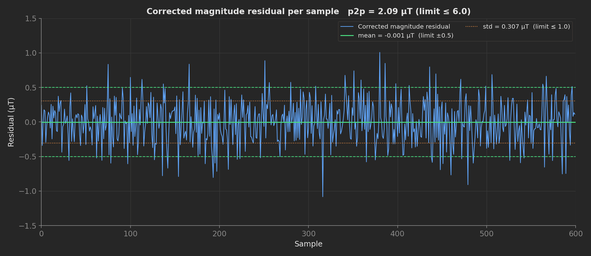
Residual per sample with the mean, std and peak-to-peak aggregations validated against their limits.
These limits start from the chip datasheet, with one subtlety worth knowing: the ±300 µT hard-iron limit assumes the sensor runs on a wide range. On a QMC5883L, the ±2 Gauss (±200 µT) range would saturate before the limit is reached, so production streaming must use the ±8 Gauss range. Limits then tighten over time as TofuPilot's control charts reveal the actual process distribution. Any unit outside 3σ but inside the absolute limits is flagged for engineering review without failing the test.
Saving Calibration to DUT
Validated parameters are written to the flight controller's persistent storage. On PX4 this means setting CAL_MAG0_XOFF, CAL_MAG0_YOFF, CAL_MAG0_ZOFF (hard iron) and CAL_MAG0_XSCALE, CAL_MAG0_YSCALE, CAL_MAG0_ZSCALE (diagonal soft iron) via MAVLink parameter set, persisted through the PX4 factory calibration storage. ArduPilot uses COMPASS_OFS_* and COMPASS_DIA_* / COMPASS_ODI_* for full 3x3 soft iron. The procedure must verify the write by reading back the parameters and confirming a power-cycle persists them. In this template the mock plug's save_calibration stands in for that write.