IMU Thermal Calibration

Introduction

IMU Overview

IMUs (Inertial Measurement Units) are remarkable sensors that measure the movement and orientation of the devices they are embedded in. Since the rise of smartphones, their size and cost have been drastically reduced, enabling a wide range of applications in robotics and drones, where they enable autonomous navigation and guidance.

IMUs combine a gyroscope (measuring angular velocity in °/s or rad/s) and an accelerometer (measuring linear acceleration in m/s² or g). Gyroscopes measure rotation but can drift over time, while accelerometers sense velocity changes and tilt but cannot distinguish between motion and gravity. Sensor fusion algorithms correct gyroscope drift with accelerometer data and stabilize accelerometer noise with gyroscope input, ensuring accurate motion tracking.

At the heart of an IMU is a Micro-Electro-Mechanical System (MEMS): a tiny structure, often just a few microns in size (about 1/100th the width of a human hair), that moves slightly in response to forces. These movements generate changes in voltage, which are measured by the sensor, converted into numerical data, and transmitted to your system through communication protocols such as SPI or I²C.

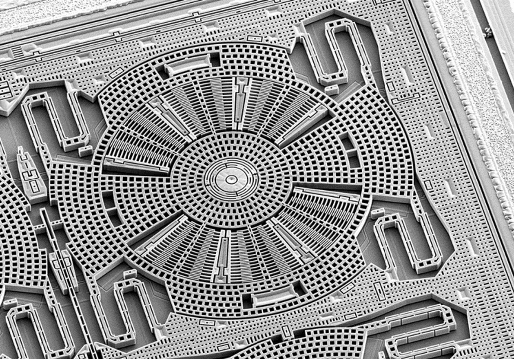
Micro-scale mechanical elements within a MEMS-based Inertial Measurement Unit (IMU).

For everyday devices like smartphones or tablets, precision isn't as important, so IMUs are not necessary factory-calibrated for temperature. But for drones and robots used in outdoor conditions, accuracy matters and calibrating the IMU for temperature can greatly improve its performance.

Calibration Purpose

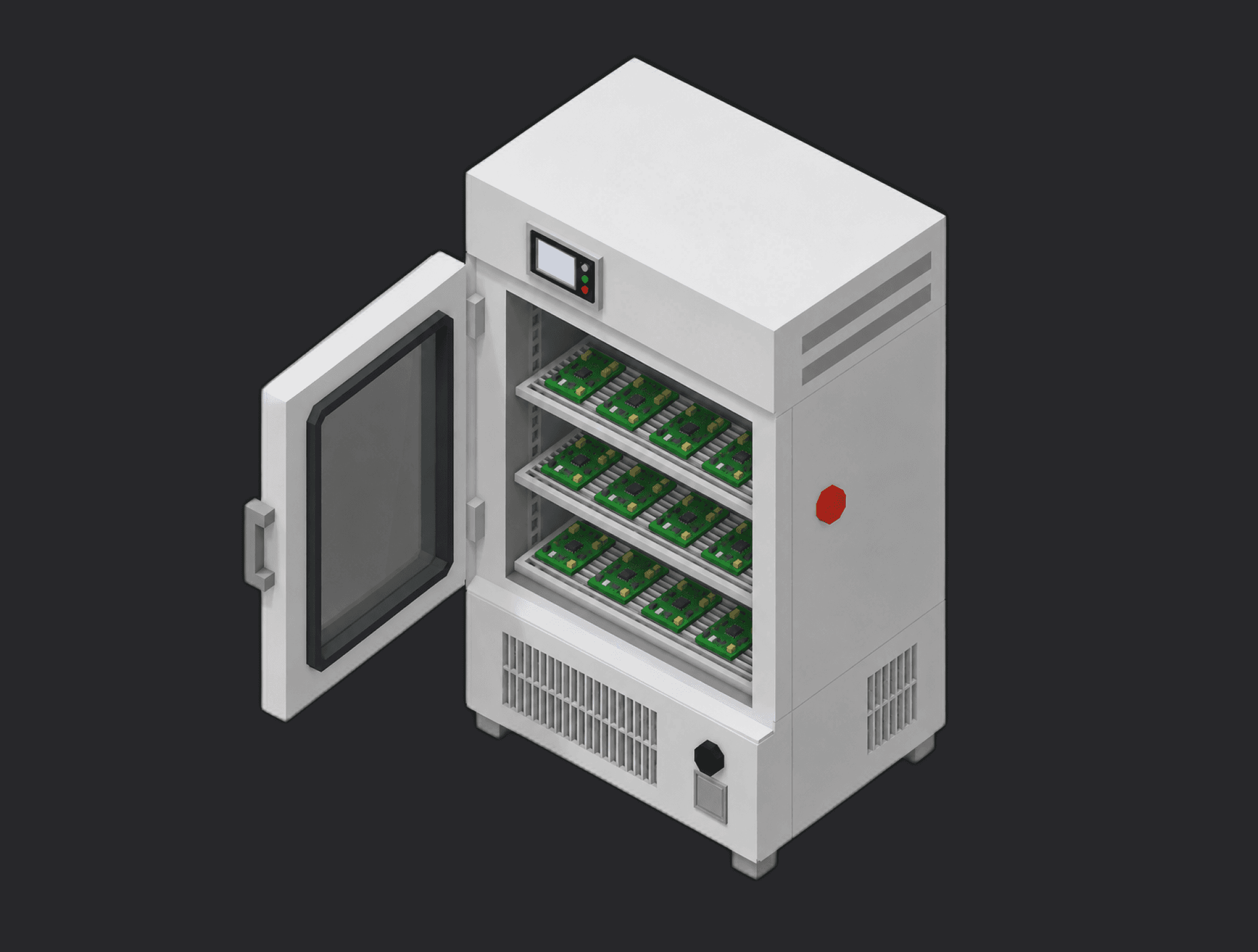
Thermal calibration involves placing the IMU-equipped Printed Circuit Board Assembly (PCBA) in a climate chamber for several hours while varying the temperature. With the IMU kept flat and motionless, any changes in its measurements are attributed to temperature effects. The resulting data is used to calculate and save calibration parameters specific to each board. During operation, these parameters are applied in real time to compensate for temperature-induced measurement variations.

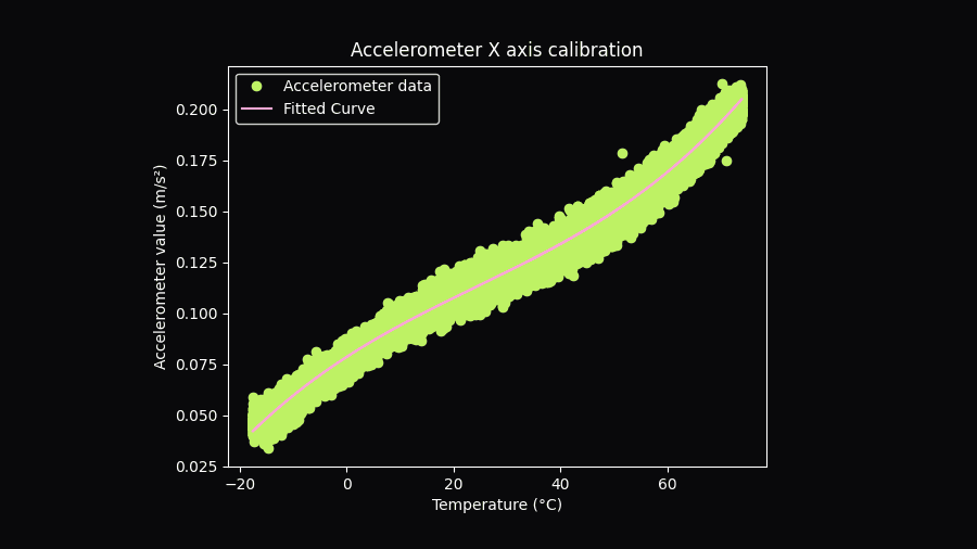
Curve showing accelerometer X vs. temperature with a polynomial fit for calibration.

Most Electronic Manufacturing Service (EMS) providers have climate chambers for tasks like stress testing, so reserving one for your boards shouldn't be an issue. For lab use, you can purchase a small climate chamber for under $5,000, suitable for testing a few boards. The cost largely depends on the chamber's temperature range. For instance, testing a drone designed for outdoor use may require a chamber that operates between -20°C and 70°C to simulate extreme environmental conditions.

Note that the temperature measured by the IMU will always be higher than the chamber's temperature due to the internal heat generated by the IMU's casing and the PCBA it is mounted on.

Equipment & Setup

To implement thermal calibration for the IMU in a drone, you will need the following:

• A climate chamber capable of reaching temperatures between -20°C and 70°C.
• A support structure to hold the PCBA in the chamber and a power supply.
• A Device Under Test (DUT), equipped with the IMU that requires calibration.
• Firmware for the device, with a triggerable mode to log the raw IMU data.
• A TofuPilot Framework procedure to:
  • Retrieve data from each board after the calibration process.
  • Calculate the calibration parameters.
  • Verify the quality of the calibration and ensure there are no defects.
  • Save the calibration parameters to the product.
• The TofuPilot Dashboard to store calibration data for traceability and analytics.

Hardware Components

Climate Chamber

We will use the Votsch VT4002 temperature test chamber, which has a temperature range of -40°C to +130°C. With its 16-liter volume, it is ideal for designing the test in the lab or for small production runs.

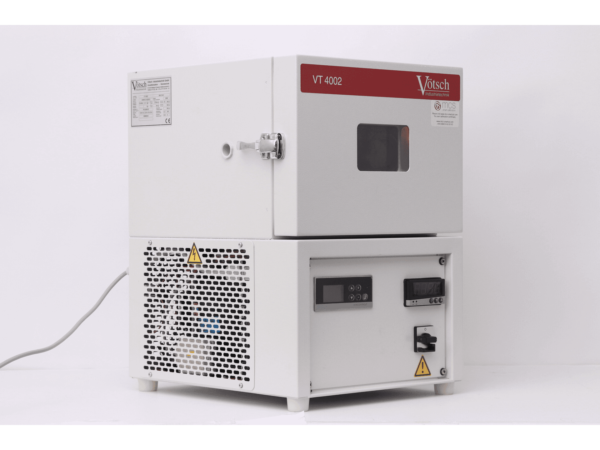
The Votsch VT4002 is a compact lab test chamber with a -40°C to +130°C range.

Cycle Program

The IMU's response is not necessarily the same when it heats up versus when it cools down. To ensure the calibration accurately reflects the sensor's real thermal behavior, we will set a calibration duration of 2 hours, with 4 temperature cycles ranging from -20°C to 70°C.

Support Structure

For the lab setup, we'll create a simple 3D-printed support using ESD filament. Foam will be added to reduce vibrations from the climate chamber. While these vibrations are likely filtered out during data processing, minimising them is still beneficial.

In mass production, we can collaborate with the test team at our EMS to design a support that accommodates multiple boards to optimise throughput, provides power to them, and is adapted to the dimensions of their temperature test chambers.

Custom Firmware

Throughout the entire calibration process, the IMU needs to log its measurements at a frequency of at least 10 Hz. To enable this, we will develop a special logging mode in the firmware. When activated, this mode will start data acquisition and record the following parameters:

• Timestamp: To track when each measurement was taken.
• Gyroscope data: X, Y, and Z axes in degrees per second (deg/s).
• Accelerometer data: X, Y, and Z axes in meters per second squared (m/s²).
• Internal sensor temperature: This will be used as the reference for calibration.

The logged data can be stored as a JSON or CSV file in the PCBA memory or on an SD card. Most climate chambers have an external pin that activates at program start. Connecting this pin to a stabilized power supply outside the chamber allows the supply to switch on automatically at the program's start and off at its end, ensuring logging occurs only during the thermal cycle and not afterward, such as when the operator retrieves the board.

Test Procedure

Overview

Once the thermal cycle is complete, the chamber powers off and the log file is ready for retrieval and processing. Operators will remove the PCBAs from their calibration support and connect them to the test station. At this point, the TofuPilot procedure takes over to:

1. Connect to the Device Under Test (DUT) and retrieve the acquisition file.
2. Validate the acquired data (noise density, temperature sensitivity).
3. Compute the polynomial calibration.
4. Validate the calibration quality (residuals, R²).
5. Save calibration results to the DUT internal memory.
6. Provide a global pass/fail status.
7. Stream results to TofuPilot for traceability and analytics.

Why TofuPilot Framework?

TofuPilot Framework is a YAML + Python test framework built for hardware manufacturing. Instead of writing all your test logic, measurements, and limits inside Python code, you describe what the test does in a procedure.yaml file, and how in small Python phase files. The framework handles:

• Automatic Python environment management (via uv)
• Operator UI (no frontend code needed)
• Measurement validation and live charts
• Process isolation between phases and equipment plugs

Project Structure

The whole procedure is six small files plus the data sample:

You can find the full source on GitHub.

The Procedure File

procedure.yaml is the entry point. It declares:

• The unit being tested (auto-identified here, so the run starts without operator input)
• A plug (Mock DUT) that simulates the board
• Two phases: Connect DUT and Thermal Calibration
• All the measurements with their limits

Here's the top of the file:

name: IMU Thermal Calibrationversion: 0.1.0description: Computes per-axis polynomial thermal compensation for an IMU's accelerometer and gyroscope, then validates fit quality.unit:  auto_identify: true  serial_number:    default_value: "SN00001"  part_number:    default_value: "PCB01"plugs:  - name: Mock DUT    description: Simulated device under test that returns logged IMU CSV data.    python: plugs.mock_dut:MockDut    key: dutmain:  - name: Connect DUT    key: connect_dut    python: phases.connect_dut  - name: Thermal Calibration    key: thermal_calibration    python: phases.thermal_calibration    depends_on:      - connect_dut

python: plugs.mock_dut:MockDut tells TofuPilot to instantiate the MockDut class. python: phases.connect_dut tells it to call the connect_dut() function in that file. The order of phases is enforced by depends_on.

Mock DUT Plug

A plug is a persistent Python class for a device or service. The framework creates it once at the start of the run and tears it down at the end. For this template we use a mock that reads a CSV file instead of talking to real hardware:

import timefrom pathlib import Pathimport pandas as pdCSV_PATH = Path(__file__).resolve().parent.parent / "data" / "imu_raw_data.csv"class MockDut:    """Simulated DUT that returns IMU log data from a CSV file."""    def __init__(self):        self._connected = False        print("Mock DUT initialized")    def connect(self) -> bool:        print("Connecting to mock DUT...")        time.sleep(0.2)        self._connected = True        return True    def get_imu_data(self) -> dict:        df = pd.read_csv(CSV_PATH, delimiter="\t")        return {            "acc_data": {                "temperature": df["imu.temperature"].tolist(),                "acc_x": df["imu.acc.x"].tolist(),                "acc_y": df["imu.acc.y"].tolist(),                "acc_z": (df["imu.acc.z"] - 9.80600).tolist(),            },            "gyro_data": {                "temperature": df["imu.temperature"].tolist(),                "gyro_x": df["imu.gyro.x"].tolist(),                "gyro_y": df["imu.gyro.y"].tolist(),                "gyro_z": df["imu.gyro.z"].tolist(),            },        }    def save_accelerometer_calibration(self, coefficients: dict) -> None:        print(f"Saved accelerometer calibration: {list(coefficients.keys())}")    def save_gyroscope_calibration(self, coefficients: dict) -> None:        print(f"Saved gyroscope calibration: {list(coefficients.keys())}")

To run against a real board, swap this class for one that talks to your firmware (UART, USB CDC, network). The rest of the pipeline stays the same.

Connect Phase

The first phase is a one-liner. The framework injects the dut plug and a log object by matching parameter names:

def connect_dut(dut, log):    log.info("Connecting to DUT...")    dut.connect()    log.info("DUT connected")

Calibration Phase

The second phase does the real work. It retrieves the IMU log, validates it, fits per-axis polynomials, validates the fit quality, and saves the result. The framework automatically passes dut, measurements, and log based on the function signature:

import numpy as npfrom utils.calibrate_sensor import calibrate_sensorfrom utils.compute_noise_density import compute_noise_densityfrom utils.compute_r2 import compute_r2from utils.compute_residuals import compute_residualsfrom utils.compute_temp_sensitivity import compute_temp_sensitivitydef thermal_calibration(dut, measurements, log):    """Retrieve IMU data, validate it, compute polynomial thermal calibration, validate fit, save."""    log.info("Fetching IMU log from DUT")    data = dut.get_imu_data()    axes = ("x", "y", "z")    calibration_results = {}    for sensor, data_key in (("acc", "acc_data"), ("gyro", "gyro_data")):        sensor_data = data[data_key]        temperature = np.asarray(sensor_data["temperature"], dtype=float)        axes_data = {axis: np.asarray(sensor_data[f"{sensor}_{axis}"], dtype=float) for axis in axes}        # --- Raw-data validation ---        for axis, values in axes_data.items():            noise = compute_noise_density(values)            sens = compute_temp_sensitivity(values, temperature)            setattr(measurements, f"{sensor}_noise_density_{axis}", noise)            setattr(measurements, f"{sensor}_temp_sensitivity_ref_{axis}", sens["sensitivity_at_ref"])        # --- Polynomial calibration ---        fit = calibrate_sensor((temperature, *axes_data.values()))        calibration_results[sensor] = {            axis: fit["polynomial_coefficients"][f"{axis}_axis"].tolist() for axis in axes        }        # --- Multi-dimensional chart per axis: raw / fitted / residual vs temperature ---        order = np.argsort(temperature)        temp_sorted = temperature[order]        for axis in axes:            raw = axes_data[axis][order]            fitted = fit["fitted_values"][f"{axis}_axis"][order]            residuals_dict = compute_residuals(raw, fitted)            md = getattr(measurements, f"{sensor}_calibration_{axis}")            md.x_axis = temp_sorted.tolist()            md.y_axis.raw = raw.tolist()            md.y_axis.fitted = fitted.tolist()            md.y_axis.residual = residuals_dict["residuals"].tolist()            aggs = md.y_axis.residual.aggregations            aggs.mean = residuals_dict["mean_residual"]            aggs.std = residuals_dict["std_residual"]            aggs.p2p = residuals_dict["p2p_residual"]            setattr(measurements, f"{sensor}_r2_{axis}", compute_r2(raw, fitted))    log.info("Saving calibration to DUT")    dut.save_accelerometer_calibration(calibration_results["acc"])    dut.save_gyroscope_calibration(calibration_results["gyro"])

The pattern is the same for every measurement: compute a value, write it to measurements. The framework matches it back to the YAML declaration and validates it.

Numeric Measurements

Each scalar measurement is declared in procedure.yaml with a name, unit, and validators. Validators express the pass/fail limits:

measurements:  - name: Acc Noise Density X    key: acc_noise_density_x    unit: m/s²/√Hz    validators:      - {operator: ">=", expected_value: 0.0}      - {operator: "<=", expected_value: 0.003}

In Python you simply assign:

The dashboard automatically renders each measurement with its limits, value, and pass/fail outcome. As more units are tested, 3 sigma limits can be computed automatically from production data on the procedure analytics page.

Multi-Dimensional Measurements

For each sensor axis, we capture the raw data, the fitted curve, and the residuals as a single multi-dimensional measurement. This replaces the static PNG plots you would otherwise have to attach manually:

- name: Acc Calibration X  key: acc_calibration_x  title: Accelerometer X vs Temperature  description: Raw accelerometer X readings vs internal temperature, with fitted 3rd-order polynomial and residuals.  x_axis: {legend: Temperature, unit: "°C"}  y_axis:    - {legend: Raw, key: raw, unit: "m/s²"}    - {legend: Fitted, key: fitted, unit: "m/s²"}    - legend: Residual      key: residual      unit: "m/s²"      aggregations:        - type: mean          validators:            - {operator: ">=", expected_value: -0.01}            - {operator: "<=", expected_value: 0.01}        - type: std          validators:            - {operator: "<=", expected_value: 5.0}        - type: p2p          validators:            - {operator: "<=", expected_value: 15.0}

Three things to notice:

1. x_axis / y_axis describe the chart. The dashboard renders an interactive plot — no need to generate or attach a PNG.
2. aggregations compute statistics over an axis (mean, standard deviation, peak-to-peak) and validate them. Here the residual mean must be near zero, the standard deviation small, and the peak-to-peak bounded.
3. R² (declared separately as a numeric measurement) catches a globally poor fit.

In Python, you set the data with intuitive attribute access:

md = measurements.acc_calibration_xmd.x_axis = temperaturesmd.y_axis.raw = raw_valuesmd.y_axis.fitted = fitted_valuesmd.y_axis.residual = residualsaggs = md.y_axis.residual.aggregationsaggs.mean = residual_meanaggs.std = residual_stdaggs.p2p = residual_p2p

Polynomial Calibration

The calibration logic itself lives in utils/calibrate_sensor.py and uses a 3rd-order polynomial fit per axis. The coefficients replace the need for large lookup tables and are programmed into the device for real-time correction:

import numpy as npdef calibrate_sensor(data, polynomial_order: int = 3):    """Fit a polynomial model per axis. Returns coefficients and fitted values."""    temp, *sensor_data = (np.asarray(arr, dtype=float) for arr in data)    poly_coeffs = {}    fitted_values = {}    axis_list = ("x", "y", "z")    for i, axis_data in enumerate(sensor_data):        axis_name = f"{axis_list[i]}_axis"        coeffs = np.polyfit(temp, axis_data, polynomial_order)        poly_coeffs[axis_name] = coeffs        fitted_values[axis_name] = np.polyval(coeffs, temp)    return {        "polynomial_coefficients": poly_coeffs,        "fitted_values": fitted_values,    }

Calibration Validation

Residuals

After fitting, we compute the residuals (the difference between the model's prediction and the actual measurements) and validate three statistics:

• mean to detect systematic bias
• std to detect variability across the temperature range
• peak-to-peak to bound the worst-case error

import numpy as npdef compute_residuals(data, fit_model):    residuals = np.asarray(data) - np.asarray(fit_model)    return {        "residuals": residuals,        "mean_residual": float(np.mean(residuals)),        "std_residual": float(np.std(residuals)),        "p2p_residual": float(np.ptp(residuals)),    }

Coefficient of Determination (R²)

Residual metrics focus on local accuracy. R² evaluates how well the model represents the sensor's behavior globally — close to 1 means the model explains most of the variance, near 0 means poor fit:

import numpy as npdef compute_r2(data, fit_model):    data = np.asarray(data, dtype=float)    fit_model = np.asarray(fit_model, dtype=float)    residuals = data - fit_model    total_variation = float(np.sum((data - np.mean(data)) ** 2))    if total_variation == 0.0:        return 1.0    return 1.0 - float(np.sum(residuals ** 2)) / total_variation

Database & Analytics

Sensor calibration, while complex, can be implemented quickly using TofuPilot Framework. The procedure can be developed during the validation phase of a new product and deployed in production when mass manufacturing begins. The quality of a test relies not only on the performance of the processing algorithms but also heavily on the choice of metrics used to validate the measurements. These metrics improve as more units are tested, allowing for more precise 3 sigma limits to be defined.

This is where TofuPilot's database and analytics solution become essential.

Automatic Upload

When a procedure declares a Dashboard ID in procedure.yaml, every run is uploaded automatically — including phases, measurements, multi-dimensional charts, and logs. No extra code, no output callback, no station server.

Run Page

After a run completes, a dedicated page is automatically created in your secure TofuPilot workspace. This page displays the test metadata (serial number, run date, procedure reference), the list of phases and measurements with their limits, units, duration and status, plus all the multi-dimensional charts rendered interactively.

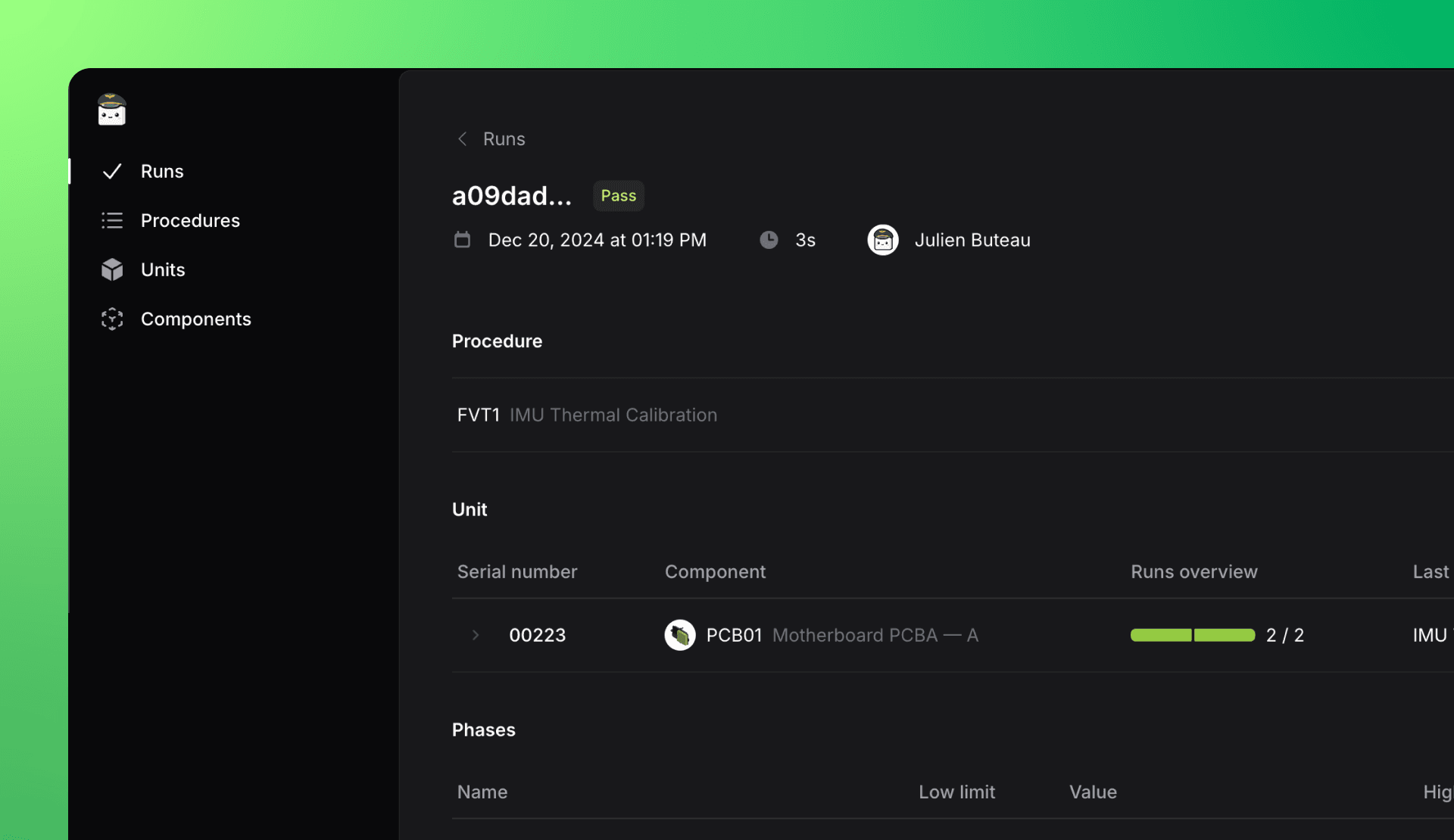
Run page displaying detailed test reports with phases and measurements.

Procedure Analytics

Analyzing the performance of a procedure across recent runs is straightforward with the procedure analytics page. Key metrics such as the run count, average test time, first pass yield, and CPK are calculated automatically. You can filter the data by date, revision, or batch to narrow down your analysis. The page also provides a detailed breakdown of performance by phase and measurement, allowing you to select a specific phase or measurement to analyze its duration, first pass yield, or CPK individually. Additionally, you can view its control chart to track recent measurements, observe trends, and determine 3 sigma values.

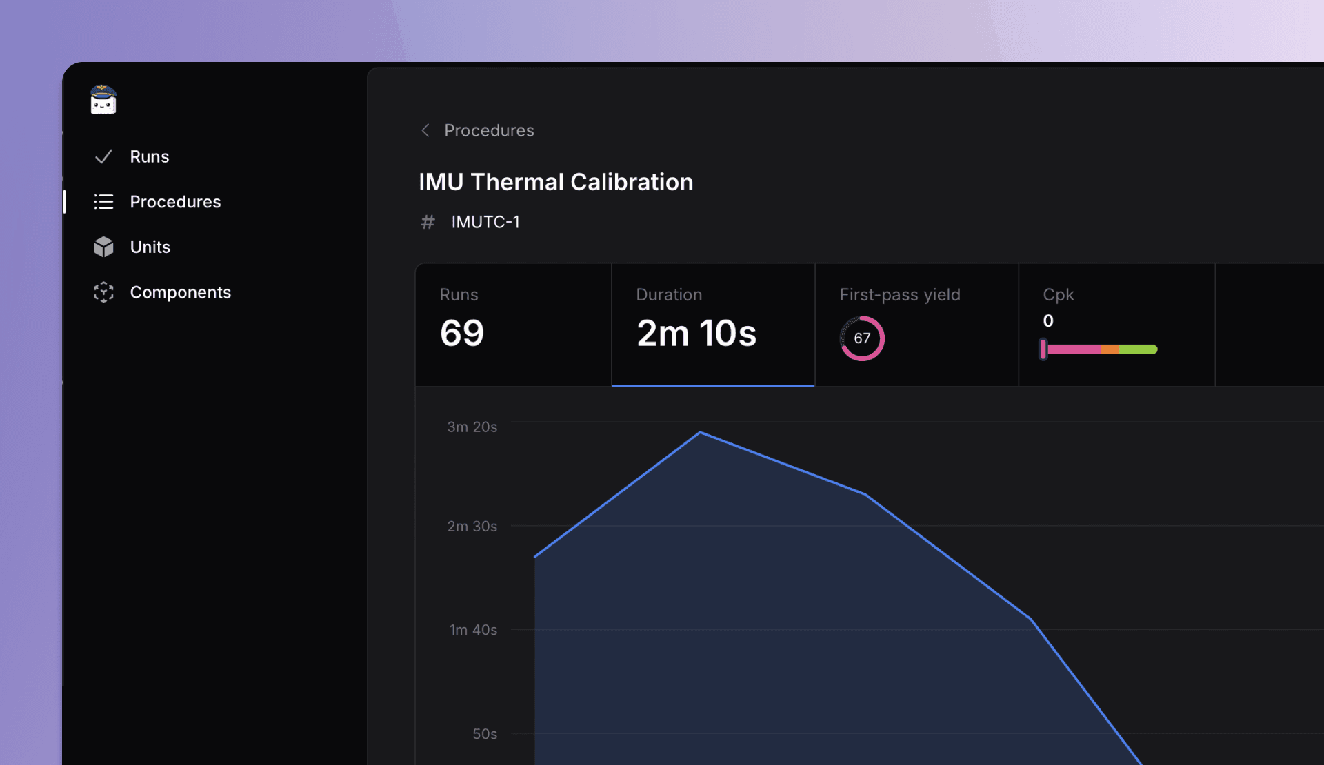
Procedure page with performance metrics, filters, and control charts.

Unit Traceability

Finally, the traceability of each tested unit is easily accessible through its dedicated page. This page provides the complete history of tests performed for the unit, any related sub-units, and a link to the page dedicated to the revision of the part.

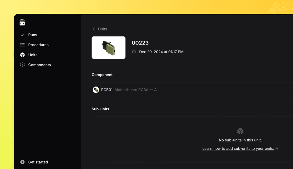
Unit page displaying the complete test history of a tested unit.